What humans see
Under a microscope, cancer looks "primitive and aggressive," a chaotic agglomeration of cells with irregularly shaped, sized, and patterned nuclei.
What computers "see"
Researchers quantified ten characteristics of cell nuclei in breast-cancer biopsy images.
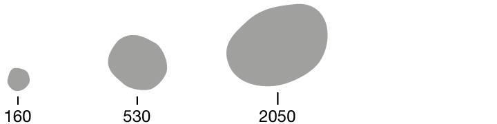
Radius
Perimeter
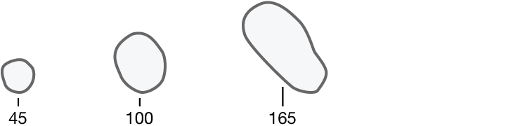
Area
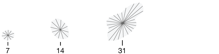
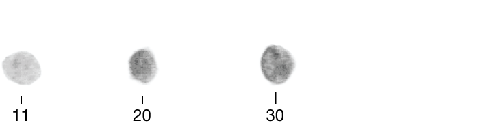
Texture
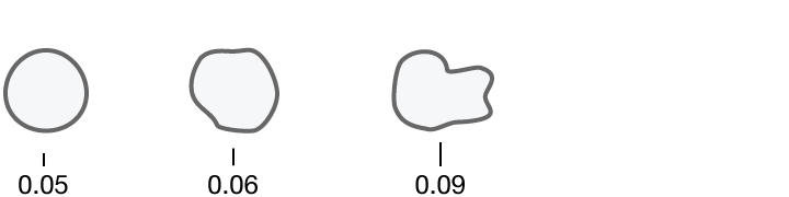
Smoothness
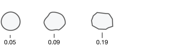
Compactness
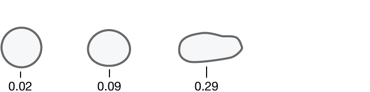
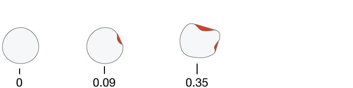
Concavity
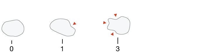
Concave Points
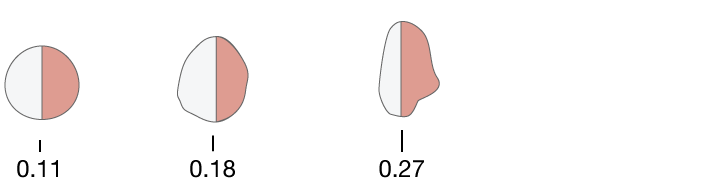
Symmetry
Fractal Dimensions